Geographic Data
A very quick introduction
Daniel Anderson
Week 9, Class 1
Learning objectives
Know the difference between vector and raster data
Be able to produce basic maps
Be able to obtain different types of geographic data from a few different places
Be able to produce basic interactive maps
Understand the basics of the R geospatial ecosystem
Today is partially about content and partially about exposure


Vector data
points, lines, and polygons
Can easily include non-spatial data (e.g., number of people living within the polygon)
- Come in the form of shapefiles (
.shp), GeoJSON, or frequently in R packages.
This is what we'll talk about almost exclusively today
Tends to be the most relevant for social science research questions

Some specific challenges with geospatial data
Coordinate reference systems and projections (we won't have much time for this)
List columns (specifically when working wtih {sf} objects)
Different geometry types (lines, points, polygons)
Vector versus raster
Data regularly stored in data "cubes" or "bricks" to represent, e.g., longitude, latitude, and elevation, or time series, or different colors
Getting spatial data
- We'll only cover a few ways to do this
Purposefully United States centric
Generally reading shape files is not terrifically difficult. Reading in and manipulating raster data can be tricky at times.
Lots of organizations out there that publish spatial data, and a fair amount are available through R packages
Working with spatial data
Two basic options
spatial
*DataFrame (from the {sp} package)sf data frame (simple features)
- We'll mostly talk about this
Working with spatial data
Two basic options
spatial
*DataFrame (from the {sp} package)sf data frame (simple features)
- We'll mostly talk about this
I can show you spatial*DataFrame outside the slides (it hung things up here). Generally, I'd stick with {sf}.
Use sf::st_as_sf to convert {sp} to {sf}
{tigris}
library(tigris)library(sf)options(tigris_class = "sf")roads_laneco <- roads("OR", "Lane")roads_laneco## Simple feature collection with 20433 features and 4 fields## geometry type: LINESTRING## dimension: XY## bbox: xmin: -124.1536 ymin: 43.4376 xmax: -121.8078 ymax: 44.29001## geographic CRS: NAD83## # A tibble: 20,433 x 5## LINEARID FULLNAME RTTYP MTFCC geometry## <chr> <chr> <chr> <chr> <LINESTRING [°]>## 1 1102152610459 W Lone Oak Lp M S1640 (-123.1256 44.10108, -123.1262 …## 2 1102217699747 Sheldon Village Lp M S1640 (-123.0742 44.07891, -123.073 4…## 3 110458663505 Cottage Hts Lp M S1400 (-123.0522 43.7893, -123.0522 4…## 4 1102152615811 Village Plz Lp M S1640 (-123.1051 44.08716, -123.1058 …## 5 110458661289 River Pointe Lp M S1400 (-123.0864 44.10306, -123.0852 …## 6 1102217699746 Sheldon Village Lp M S1640 (-123.0723 44.07875, -123.0723 …## 7 110458664549 Village Plz Lp M S1400 (-123.1053 44.08658, -123.1052 …## 8 1102223141058 Carpenter Byp M S1400 (-123.3368 43.78013, -123.3367 …## 9 1106092829172 State Hwy 126 Bus S S1200 (-123.0502 44.04391, -123.0502 …## 10 1104493105112 State Hwy 126 Bus S S1200 (-122.996 44.04587, -122.9959 4…## # … with 20,423 more rowsI/O
Let's say I want to write the file to disk.
# from the sf librarywrite_sf(roads_laneco, here::here("data", "roads_lane.shp"))Then read it in later
roads_laneco <- read_sf(here::here("data", "roads_lane.shp"))roads_laneco## Simple feature collection with 20433 features and 4 fields## geometry type: LINESTRING## dimension: XY## bbox: xmin: -124.1536 ymin: 43.4376 xmax: -121.8078 ymax: 44.29001## geographic CRS: NAD83## # A tibble: 20,433 x 5## LINEARID FULLNAME RTTYP MTFCC geometry## <chr> <chr> <chr> <chr> <LINESTRING [°]>## 1 1102152610459 W Lone Oak Lp M S1640 (-123.1256 44.10108, -123.1262 …## 2 1102217699747 Sheldon Village Lp M S1640 (-123.0742 44.07891, -123.073 4…## 3 110458663505 Cottage Hts Lp M S1400 (-123.0522 43.7893, -123.0522 4…## 4 1102152615811 Village Plz Lp M S1640 (-123.1051 44.08716, -123.1058 …## 5 110458661289 River Pointe Lp M S1400 (-123.0864 44.10306, -123.0852 …## 6 1102217699746 Sheldon Village Lp M S1640 (-123.0723 44.07875, -123.0723 …## 7 110458664549 Village Plz Lp M S1400 (-123.1053 44.08658, -123.1052 …## 8 1102223141058 Carpenter Byp M S1400 (-123.3368 43.78013, -123.3367 …## 9 1106092829172 State Hwy 126 Bus S S1200 (-123.0502 44.04391, -123.0502 …## 10 1104493105112 State Hwy 126 Bus S S1200 (-122.996 44.04587, -122.9959 4…## # … with 20,423 more rows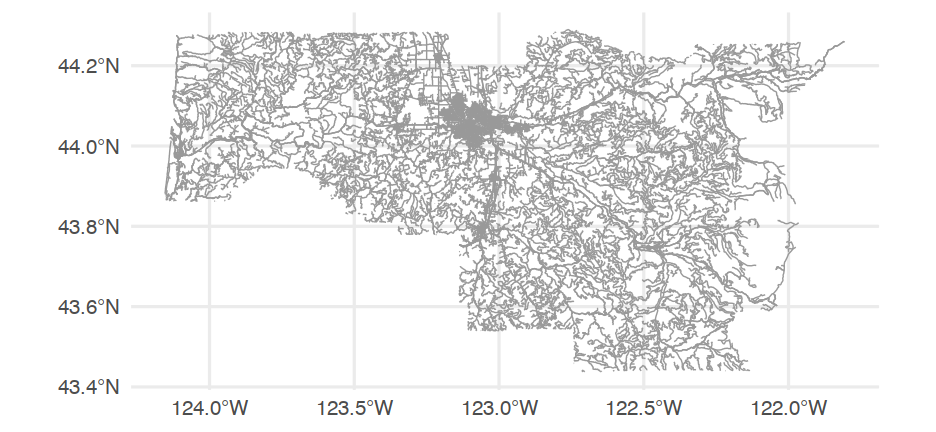
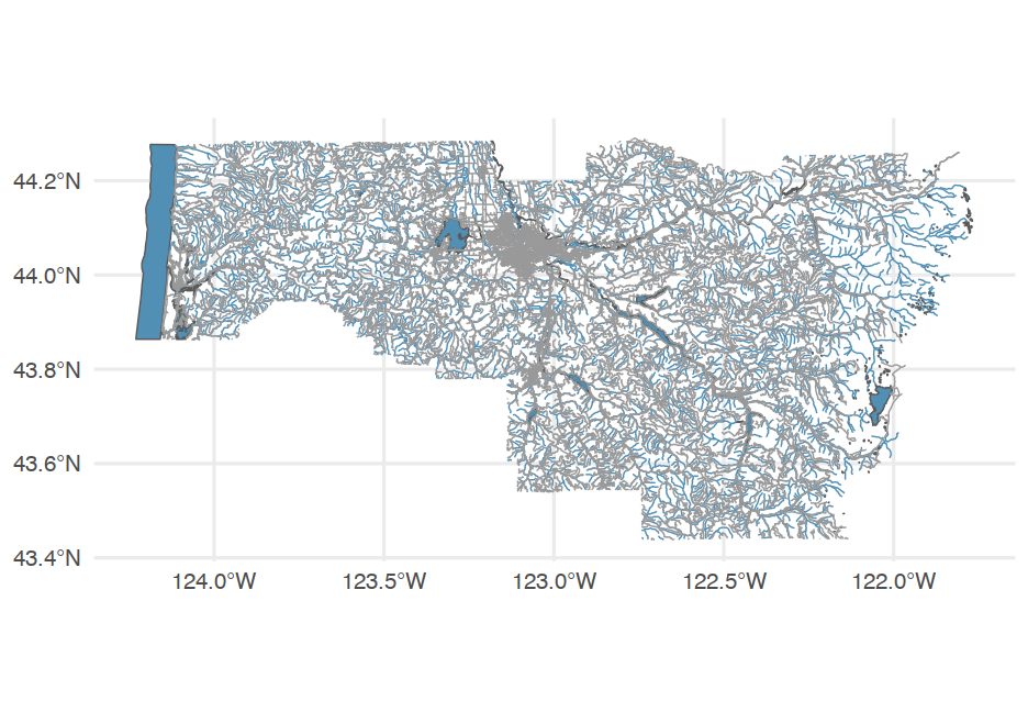
Add water features
lakes <- area_water("OR", "Lane")streams <- linear_water("OR", "Lane")ggplot() + geom_sf(data = lakes, fill = "#518FB5") + # Add lakes geom_sf(data = streams, color = "#518FB5") + # Add streams/drainage geom_sf(data = roads_laneco, color = "gray60") # add roadsNote - these functions are all from the {tigris} package.
Quick aside
Similar package osmdata
- Specifically for street-level data.
- We'll just use the boundry box functionality, but you can add many of the same things (and there are other packages that will provide you with boundary boxes)
bb <- osmdata::getbb("Eugene")bb## min max## x -123.20876 -123.03589## y 43.98753 44.13227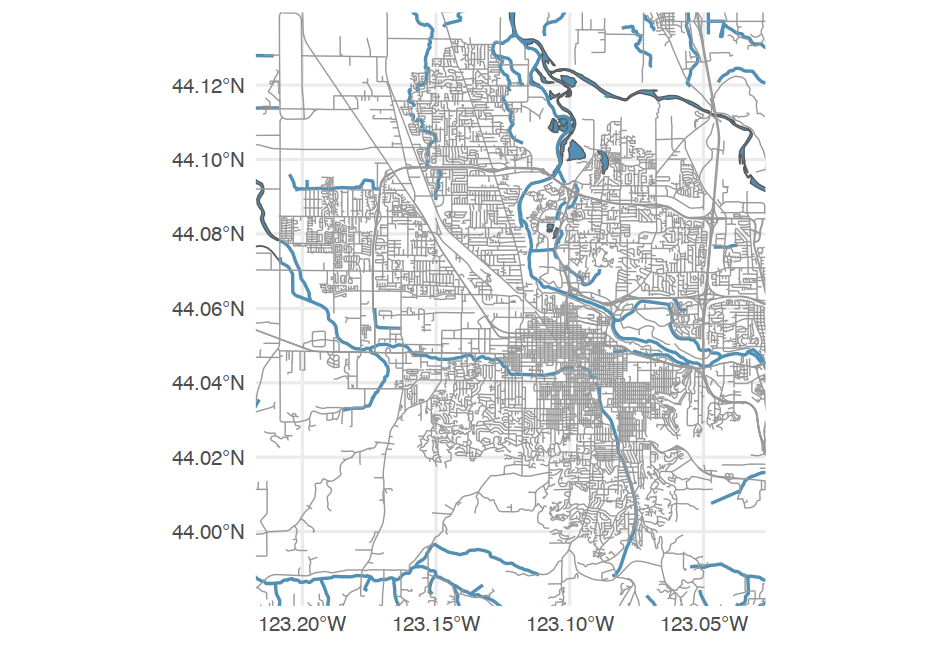
Use the data to plot
ggplot() + geom_sf(data = water$osm_multipolygons, fill = "#518FB5", color = darken("#518FB5")) + geom_sf(data = water$osm_polygons, fill = "#518FB5", color = darken("#518FB5")) + geom_sf(data = water$osm_lines, color = darken("#518FB5")) + geom_sf(data = roads$osm_lines, color = "gray40", size = 0.2) + coord_sf(xlim = bb[1, ], ylim = bb[2, ], expand = FALSE) + labs(caption = "Eugene, OR")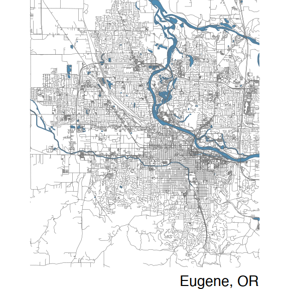
Let's get some census data
Note
To do this, you need to first register an API key with the US Census,
which you can do here. Then
use census_api_key("YOUR API KEY").
Alternatively, you can specify CENSUS_API_KEY = "YOUR API KEY"
in .Renviron. You can do this by using usethis::edit_r_environ()
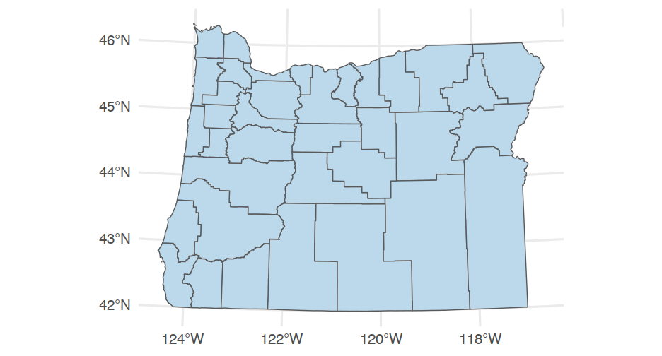
Getting the data
library(tidycensus)# Find variable code# v <- load_variables(2018, "acs5")# View(v)census_vals <- get_acs(geography = "tract", state = "OR", variables = c(med_income = "B06011_001", ed_attain = "B15003_001"), year = 2018, geometry = TRUE)## | | | 0% | | | 1% | |= | 1% | |= | 2% | |== | 2% | |== | 3% | |=== | 4% | |=== | 5% | |==== | 5% | |==== | 6% | |===== | 6% | |===== | 7% | |===== | 8% | |====== | 8% | |====== | 9% | |======= | 9% | |======= | 10% | |======== | 11% | |======== | 12% | |========= | 13% | |========== | 14% | |========== | 15% | |=========== | 16% | |============ | 17% | |============ | 18% | |============= | 19% | |============== | 20% | |======================== | 34% | |========================= | 35% | |========================== | 37% | |=========================== | 38% | |============================ | 40% | |============================= | 41% | |============================== | 43% | |=============================== | 45% | |================================ | 46% | |================================= | 47% | |================================= | 48% | |================================== | 49% | |==================================== | 51% | |===================================== | 52% | |====================================== | 54% | |======================================= | 55% | |======================================== | 57% | |================================================ | 68% | |================================================= | 69% | |================================================= | 70% | |================================================== | 72% | |=================================================== | 73% | |==================================================== | 74% | |===================================================== | 76% | |====================================================== | 77% | |======================================================= | 79% | |======================================================== | 80% | |========================================================= | 82% | |=========================================================== | 84% | |============================================================ | 86% | |============================================================= | 87% | |============================================================== | 89% | |=============================================================== | 91% | |================================================================ | 92% | |================================================================== | 94% | |=================================================================== | 96% | |======================================================================| 100%Look at the data
census_vals## Simple feature collection with 1668 features and 5 fields (with 12 geometries empty)## geometry type: MULTIPOLYGON## dimension: XY## bbox: xmin: -124.5662 ymin: 41.99179 xmax: -116.4635 ymax: 46.29204## geographic CRS: NAD83## First 10 features:## GEOID NAME variable estimate## 1 41045970600 Census Tract 9706, Malheur County, Oregon med_income 23670## 2 41045970600 Census Tract 9706, Malheur County, Oregon ed_attain 2714## 3 41047001200 Census Tract 12, Marion County, Oregon med_income 27106## 4 41047001200 Census Tract 12, Marion County, Oregon ed_attain 2695## 5 41047002000 Census Tract 20, Marion County, Oregon med_income 33271## 6 41047002000 Census Tract 20, Marion County, Oregon ed_attain 7260## 7 41047010501 Census Tract 105.01, Marion County, Oregon med_income 31291## 8 41047010501 Census Tract 105.01, Marion County, Oregon ed_attain 4099## 9 41051000301 Census Tract 3.01, Multnomah County, Oregon med_income 22531## 10 41051000301 Census Tract 3.01, Multnomah County, Oregon ed_attain 3550## moe geometry## 1 3812 MULTIPOLYGON (((-117.4678 4...## 2 211 MULTIPOLYGON (((-117.4678 4...## 3 5112 MULTIPOLYGON (((-123.0447 4...## 4 213 MULTIPOLYGON (((-123.0447 4...## 5 3565 MULTIPOLYGON (((-123.0362 4...## 6 477 MULTIPOLYGON (((-123.0362 4...## 7 5080 MULTIPOLYGON (((-122.7894 4...## 8 363 MULTIPOLYGON (((-122.7894 4...## 9 3680 MULTIPOLYGON (((-122.6435 4...## 10 436 MULTIPOLYGON (((-122.6435 4...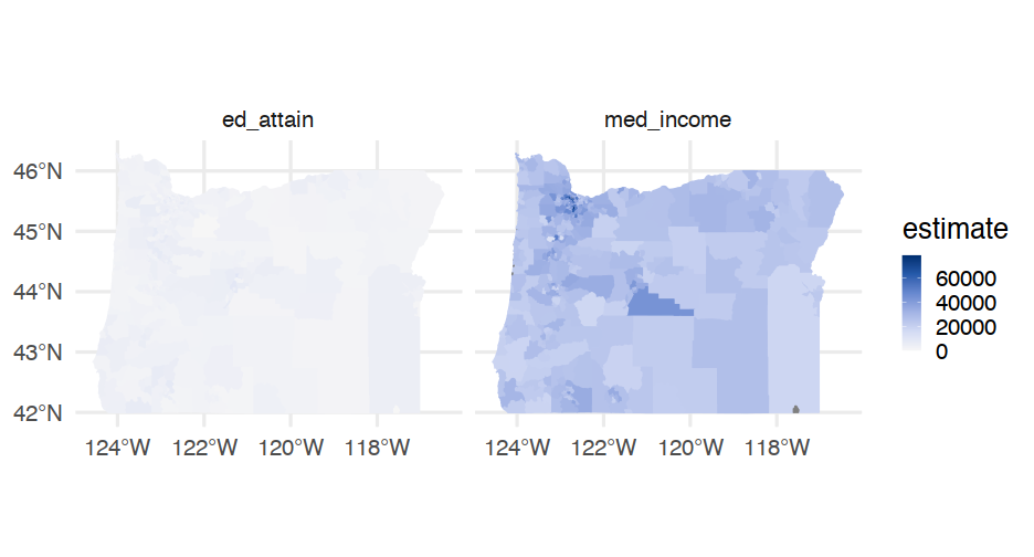
Try again
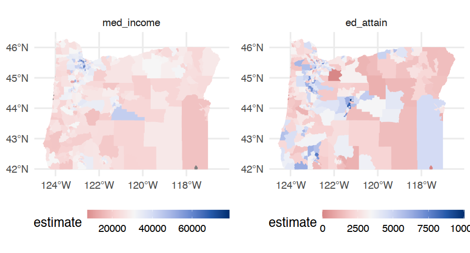
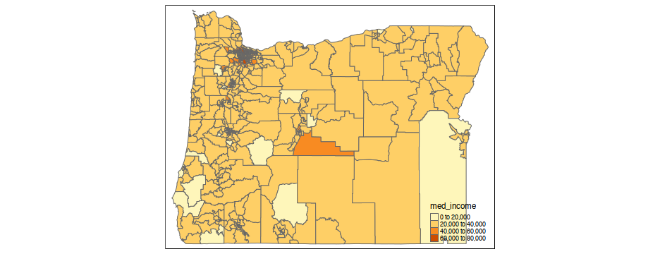
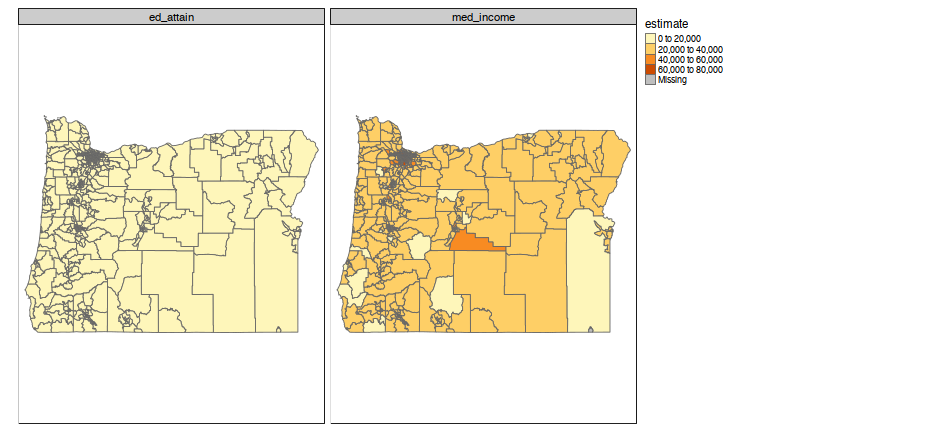
library(colorspace)income <- filter(census_vals, variable == "med_income")income_plot <- ggplot(income) + geom_sf(aes(fill = estimate, color = estimate)) + facet_wrap(~variable) + guides(color = "none") + scale_fill_continuous_diverging( "Blue-Red 3", rev = TRUE, mid = mean(income$estimate, na.rm = TRUE) ) + scale_color_continuous_diverging( "Blue-Red 3", rev = TRUE, mid = mean(income$estimate, na.rm = TRUE) ) + theme(legend.position = "bottom", legend.key.width = unit(2, "cm"))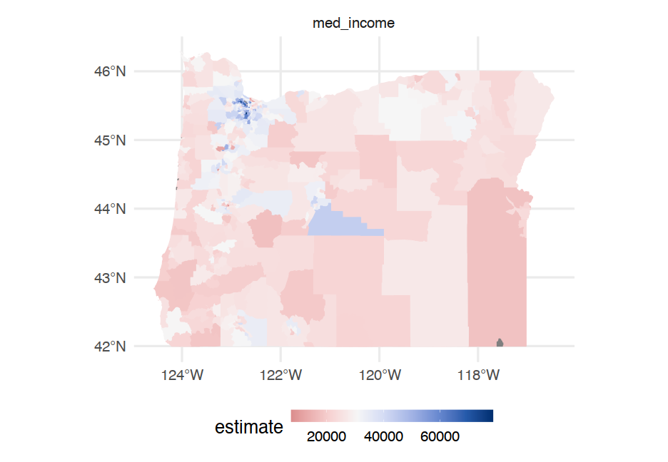
Same thing for education
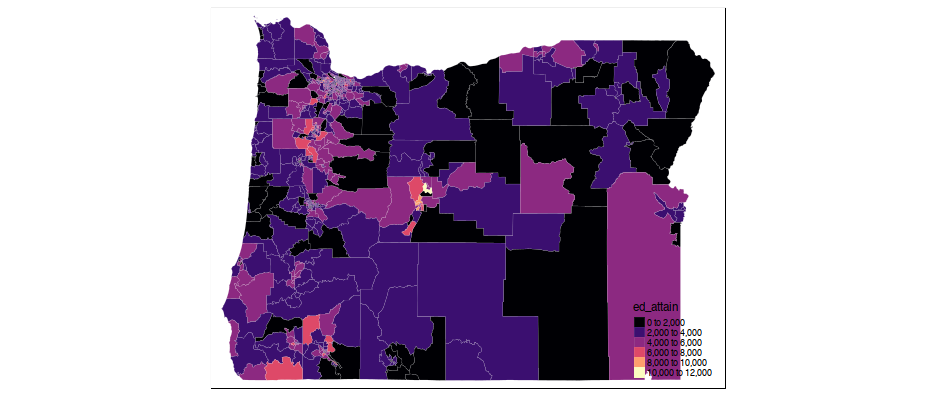
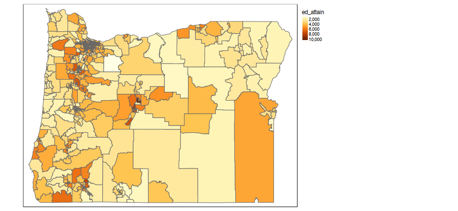
ed <- filter(census_vals, variable == "ed_attain")ed_plot <- ggplot(ed) + geom_sf(aes(fill = estimate, color = estimate)) + facet_wrap(~variable) + guides(color = "none") + scale_fill_continuous_diverging( "Blue-Red 3", rev = TRUE, mid = mean(ed$estimate, na.rm = TRUE) ) + scale_color_continuous_diverging( "Blue-Red 3", rev = TRUE, mid = mean(ed$estimate, na.rm = TRUE) ) + theme(legend.position = "bottom", legend.key.width = unit(2, "cm"))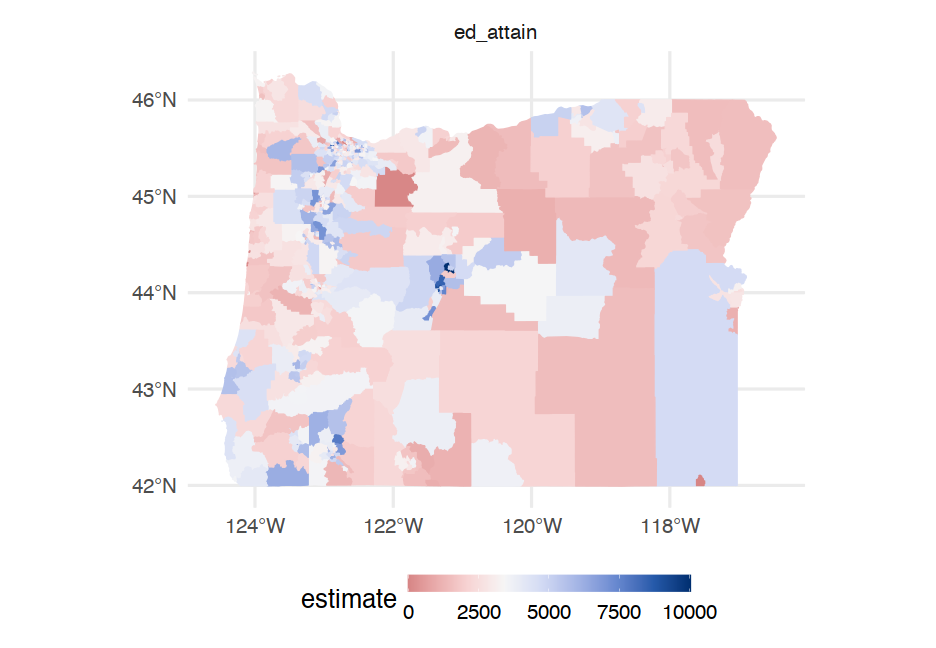
How?
There are a few different ways. Here's one:
Break continuous variable into categorical values
Assign each combination of values between categorical vars a color
Make sure the combinations of the colors make sense
gif from Joshua Stevens
Do it
Note - this will be fairly quick. I'm not expecting you to know how to do this, but I want to show you the idea and give you the breadcrumbs for the code you may need.
First - move it to wider
wider <- census_vals %>% select(-moe) %>% spread(variable, estimate) %>% # pivot_wider doesn't work w/sf yet drop_na(ed_attain, med_income)wider## Simple feature collection with 825 features and 4 fields## geometry type: MULTIPOLYGON## dimension: XY## bbox: xmin: -124.5662 ymin: 41.99179 xmax: -116.4635 ymax: 46.29204## geographic CRS: NAD83## First 10 features:## GEOID NAME ed_attain med_income## 1 41001950100 Census Tract 9501, Baker County, Oregon 2228 24846## 2 41001950200 Census Tract 9502, Baker County, Oregon 2374 23288## 3 41001950300 Census Tract 9503, Baker County, Oregon 1694 24080## 4 41001950400 Census Tract 9504, Baker County, Oregon 2059 24083## 5 41001950500 Census Tract 9505, Baker County, Oregon 1948 26207## 6 41001950600 Census Tract 9506, Baker County, Oregon 1604 23381## 7 41003000100 Census Tract 1, Benton County, Oregon 5509 26188## 8 41003000202 Census Tract 2.02, Benton County, Oregon 3630 35343## 9 41003000400 Census Tract 4, Benton County, Oregon 5562 40869## 10 41003000500 Census Tract 5, Benton County, Oregon 2526 38922## geometry## 1 MULTIPOLYGON (((-118.5194 4...## 2 MULTIPOLYGON (((-117.9158 4...## 3 MULTIPOLYGON (((-117.9506 4...## 4 MULTIPOLYGON (((-117.8309 4...## 5 MULTIPOLYGON (((-117.9774 4...## 6 MULTIPOLYGON (((-117.7775 4...## 7 MULTIPOLYGON (((-123.2812 4...## 8 MULTIPOLYGON (((-123.3415 4...## 9 MULTIPOLYGON (((-123.3039 4...## 10 MULTIPOLYGON (((-123.2979 4...Create the cut variable
wider <- wider %>% mutate(cat_ed = cut(ed_attain, ed_quartiles), cat_inc = cut(med_income, inc_quartiles))wider %>% select(starts_with("cat"))## Simple feature collection with 825 features and 2 fields## geometry type: MULTIPOLYGON## dimension: XY## bbox: xmin: -124.5662 ymin: 41.99179 xmax: -116.4635 ymax: 46.29204## geographic CRS: NAD83## First 10 features:## cat_ed cat_inc geometry## 1 (54,2.68e+03] (7.46e+03,2.56e+04] MULTIPOLYGON (((-118.5194 4...## 2 (54,2.68e+03] (7.46e+03,2.56e+04] MULTIPOLYGON (((-117.9158 4...## 3 (54,2.68e+03] (7.46e+03,2.56e+04] MULTIPOLYGON (((-117.9506 4...## 4 (54,2.68e+03] (7.46e+03,2.56e+04] MULTIPOLYGON (((-117.8309 4...## 5 (54,2.68e+03] (2.56e+04,3.24e+04] MULTIPOLYGON (((-117.9774 4...## 6 (54,2.68e+03] (7.46e+03,2.56e+04] MULTIPOLYGON (((-117.7775 4...## 7 (3.89e+03,1e+04] (2.56e+04,3.24e+04] MULTIPOLYGON (((-123.2812 4...## 8 (2.68e+03,3.89e+03] (3.24e+04,7.86e+04] MULTIPOLYGON (((-123.3415 4...## 9 (3.89e+03,1e+04] (3.24e+04,7.86e+04] MULTIPOLYGON (((-123.3039 4...## 10 (54,2.68e+03] (3.24e+04,7.86e+04] MULTIPOLYGON (((-123.2979 4...Set palette
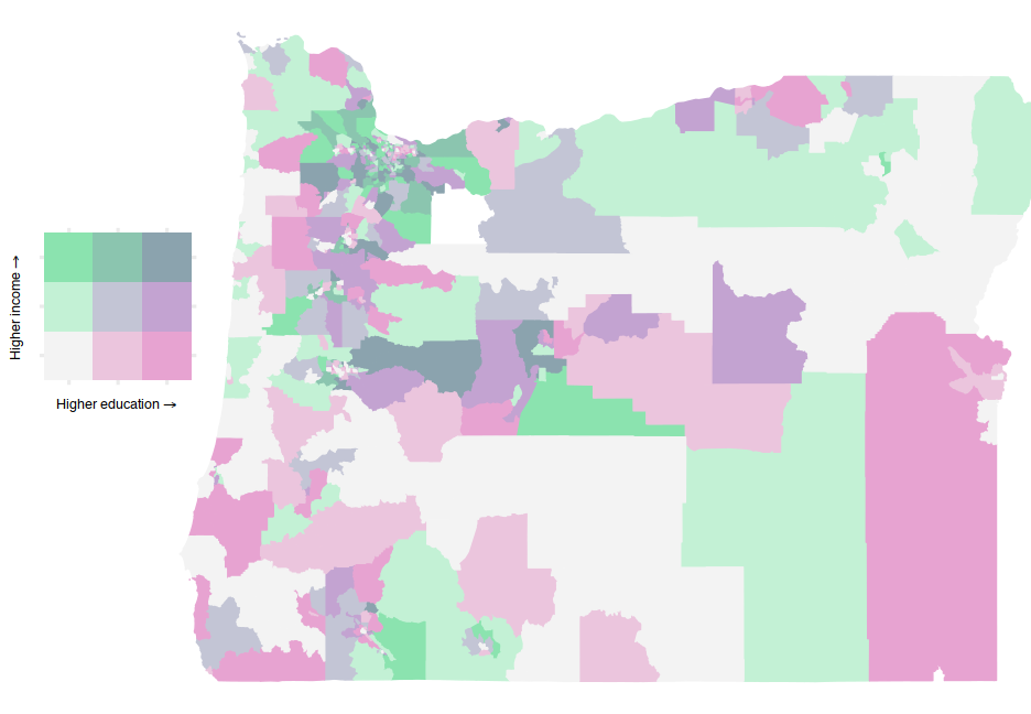
# First drop geo columnpal <- st_drop_geometry(wider) %>% count(cat_ed, cat_inc) %>% arrange(cat_ed, cat_inc) %>% drop_na(cat_ed, cat_inc) %>% mutate(pal = c("#F3F3F3", "#C3F1D5", "#8BE3AF", "#EBC5DD", "#C3C5D5", "#8BC5AF", "#E7A3D1", "#C3A3D1", "#8BA3AE"))pal## cat_ed cat_inc n pal## 1 (54,2.68e+03] (7.46e+03,2.56e+04] 113 #F3F3F3## 2 (54,2.68e+03] (2.56e+04,3.24e+04] 87 #C3F1D5## 3 (54,2.68e+03] (3.24e+04,7.86e+04] 73 #8BE3AF## 4 (2.68e+03,3.89e+03] (7.46e+03,2.56e+04] 85 #EBC5DD## 5 (2.68e+03,3.89e+03] (2.56e+04,3.24e+04] 97 #C3C5D5## 6 (2.68e+03,3.89e+03] (3.24e+04,7.86e+04] 93 #8BC5AF## 7 (3.89e+03,1e+04] (7.46e+03,2.56e+04] 75 #E7A3D1## 8 (3.89e+03,1e+04] (2.56e+04,3.24e+04] 91 #C3A3D1## 9 (3.89e+03,1e+04] (3.24e+04,7.86e+04] 109 #8BA3AE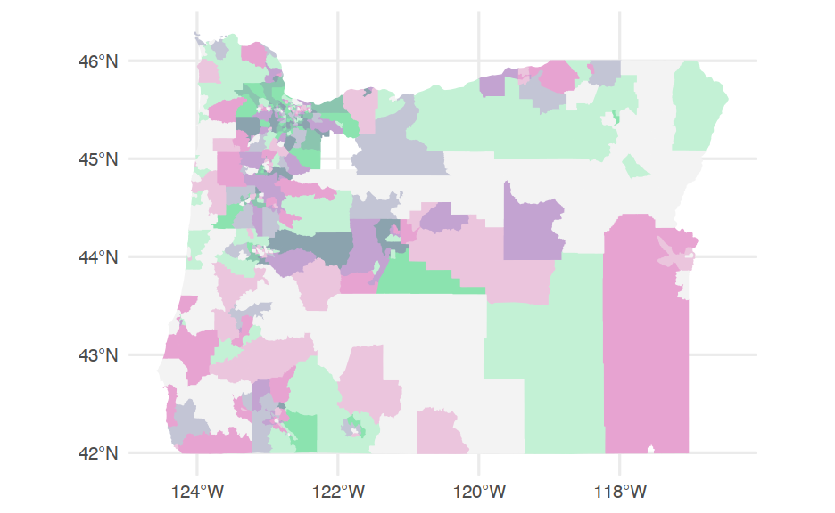
Add in legend
First create it
leg <- ggplot(pal, aes(cat_ed, cat_inc)) + geom_tile(aes(fill = pal)) + scale_fill_identity() + coord_fixed() + labs(x = expression("Higher education" %->% ""), y = expression("Higher income" %->% "")) + theme(axis.text = element_blank(), axis.title = element_text(size = 12))leg
Add text
- First, let's get data at the county level, instead of census tract level
cnty <- get_acs(geography = "county", state = "OR", variables = c(ed_attain = "B15003_001"), year = 2018, geometry = TRUE)## | | | 0% | | | 1% | |= | 1% | |= | 2% | |== | 2% | |== | 3% | |=== | 4% | |=== | 5% | |==== | 5% | |==== | 6% | |===== | 7% | |====== | 8% | |====== | 9% | |======= | 9% | |======== | 11% | |======== | 12% | |========= | 13% | |========= | 14% | |========== | 14% | |========== | 15% | |=========== | 15% | |=========== | 16% | |============ | 17% | |============ | 18% | |============= | 18% | |============= | 19% | |=============== | 22% | |================ | 22% | |================ | 23% | |================= | 24% | |================= | 25% | |================== | 25% | |================== | 26% | |=================== | 26% | |=================== | 27% | |=================== | 28% | |==================== | 28% | |==================== | 29% | |===================== | 29% | |===================== | 30% | |===================== | 31% | |====================== | 31% | |====================== | 32% | |======================= | 32% | |======================== | 35% | |========================= | 35% | |========================= | 36% | |========================== | 37% | |========================== | 38% | |=========================== | 38% | |=========================== | 39% | |============================= | 41% | |============================= | 42% | |============================== | 42% | |============================== | 43% | |=============================== | 44% | |=============================== | 45% | |================================ | 45% | |================================ | 46% | |================================= | 47% | |================================= | 48% | |================================== | 48% | |=================================== | 51% | |==================================== | 51% | |==================================== | 52% | |===================================== | 52% | |===================================== | 53% | |======================================= | 56% | |======================================== | 56% | |======================================== | 57% | |======================================== | 58% | |========================================= | 58% | |========================================= | 59% | |========================================== | 59% | |========================================== | 60% | |============================================ | 63% | |============================================= | 64% | |============================================= | 65% | |============================================== | 65% | |============================================== | 66% | |=============================================== | 67% | |=============================================== | 68% | |================================================ | 68% | |================================================ | 69% | |================================================= | 69% | |================================================= | 70% | |================================================= | 71% | |================================================== | 71% | |================================================== | 72% | |=================================================== | 72% | |=================================================== | 73% | |==================================================== | 74% | |==================================================== | 75% | |====================================================== | 78% | |======================================================= | 78% | |======================================================= | 79% | |======================================================== | 79% | |======================================================== | 80% | |======================================================== | 81% | |========================================================= | 81% | |=========================================================== | 85% | |============================================================ | 85% | |============================================================ | 86% | |============================================================= | 87% | |============================================================= | 88% | |============================================================== | 88% | |============================================================== | 89% | |=============================================================== | 90% | |=============================================================== | 91% | |================================================================ | 91% | |================================================================ | 92% | |================================================================= | 92% | |================================================================= | 93% | |================================================================= | 94% | |================================================================== | 94% | |================================================================== | 95% | |=================================================================== | 95% | |=================================================================== | 96% | |==================================================================== | 96% | |===================================================================== | 99% | |======================================================================| 99% | |======================================================================| 100%cnty## Simple feature collection with 36 features and 5 fields## geometry type: MULTIPOLYGON## dimension: XY## bbox: xmin: -124.5662 ymin: 41.99179 xmax: -116.4635 ymax: 46.29204## geographic CRS: NAD83## First 10 features:## GEOID NAME variable estimate moe## 1 41005 Clackamas County, Oregon ed_attain 285481 121## 2 41021 Gilliam County, Oregon ed_attain 1448 97## 3 41033 Josephine County, Oregon ed_attain 63006 172## 4 41035 Klamath County, Oregon ed_attain 46345 108## 5 41039 Lane County, Oregon ed_attain 251966 137## 6 41043 Linn County, Oregon ed_attain 85098 147## 7 41051 Multnomah County, Oregon ed_attain 579186 133## 8 41055 Sherman County, Oregon ed_attain 1238 73## 9 41061 Union County, Oregon ed_attain 17317 115## 10 41007 Clatsop County, Oregon ed_attain 27935 125## geometry## 1 MULTIPOLYGON (((-122.8679 4...## 2 MULTIPOLYGON (((-120.6535 4...## 3 MULTIPOLYGON (((-124.042 42...## 4 MULTIPOLYGON (((-122.29 42....## 5 MULTIPOLYGON (((-124.1503 4...## 6 MULTIPOLYGON (((-123.2608 4...## 7 MULTIPOLYGON (((-122.9292 4...## 8 MULTIPOLYGON (((-121.0312 4...## 9 MULTIPOLYGON (((-118.6978 4...## 10 MULTIPOLYGON (((-123.5989 4...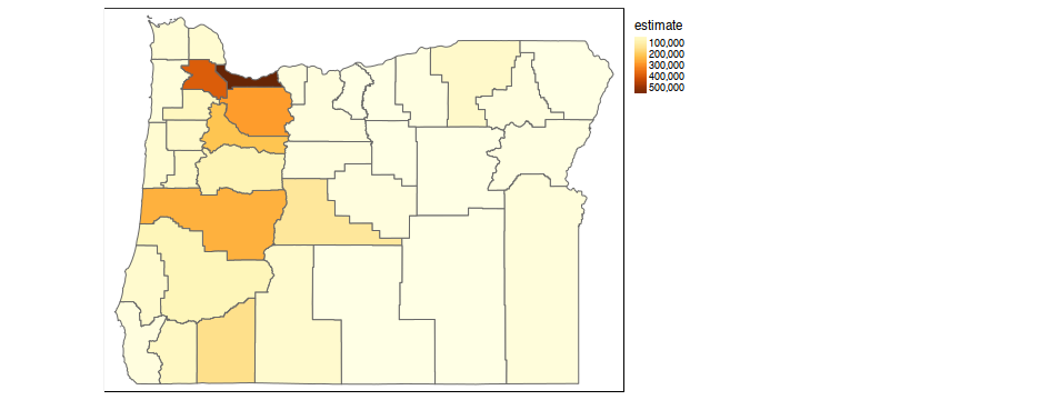
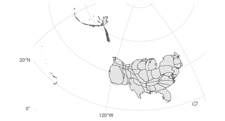
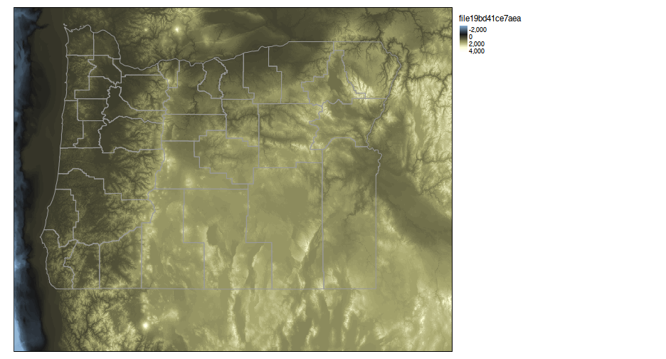
Add raster elevation data
states <- get_acs("state", variables = c(ed_attain = "B15003_001"), year = 2018, geometry = TRUE)or <- filter(states, NAME == "Oregon")# convert to spatial data framesp <- as(or, "Spatial")# use elevatr library to pull datalibrary(elevatr)or_elev <- get_elev_raster(sp, z = 9)lane_elev <- get_elev_raster(sp, z = 9)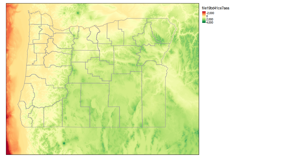

mapview
- Really quick easy interactive maps
library(mapview)mapview(cnty)


mapview(cnty, zcol = "estimate")

mapview(cnty, zcol = "estimate", popup = leafpop::popupTable(cnty, zcol = c("NAME", "estimate")))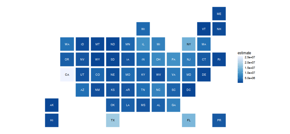
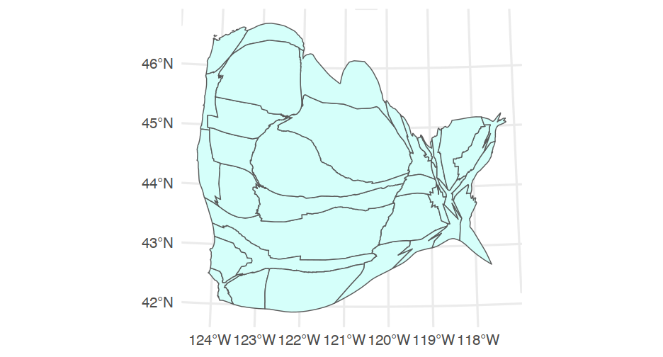
Cartograms
library(cartogram)or_county_pop <- get_acs(geography = "county", state = "OR", variables = "B00001_001", year = 2018, geometry = TRUE)# Set projectionor_county_pop <- st_transform(or_county_pop, crs = 2992) # found the CRS here: https://www.oregon.gov/geo/pages/projections.aspxcarto_counties <- cartogram_cont(or_county_pop, "estimate")