Agenda

• Tables with gt
• Fonts with showtext and/or extrafont

Learning objectives

• Be comfortable with the basics of gt
  • create a table
  • format columns
  • create spanner heads
  • etc.
• Understand how to use additional fonts (if you so choose)

Overview

• Pipe-oriented

• Beautiful tables easy

• Spanner heads/grouping used to be a total pain - not so anymore

• Renders to HTML/PDF without even thinking about it

Probably my favorite package for creating static tables, although kableExtra is great too.

My experience is that fewer people are generally familiar with gt, which is why I cover it here.

Install

install.packages("gt")
# or
remotes::install_github("rstudio/gt")

The hard part

• Getting your data in the format you want a table in

• Utilize your pivot_* skills regularly

library(fivethirtyeight)
flying

## # A tibble: 1,040 x 27
##   respondent_id gender age   height   children_under_18 household_income   
##           <dbl> <chr>  <ord> <ord>    <lgl>             <ord>              
## 1    3436139758 <NA>   <NA>   <NA>    NA                <NA>               
## 2    3434278696 Male   30-44 "6'3\""  TRUE              <NA>               
## 3    3434275578 Male   30-44 "5'8\""  FALSE             $100,000 - $149,999
## 4    3434268208 Male   30-44 "5'11\"" FALSE             $0 - $24,999       
## 5    3434250245 Male   30-44 "5'7\""  FALSE             $50,000 - $99,999  
## 6    3434245875 Male   30-44 "5'9\""  TRUE              $25,000 - $49,999  
## # … with 1,034 more rows, and 21 more variables: education <ord>,
## #   location <chr>, frequency <ord>, recline_frequency <ord>,
## #   recline_obligation <lgl>, recline_rude <ord>, recline_eliminate <lgl>,
## #   switch_seats_friends <ord>, switch_seats_family <ord>,
## #   wake_up_bathroom <ord>, wake_up_walk <ord>, baby <ord>,
## #   unruly_child <ord>, two_arm_rests <chr>, middle_arm_rest <chr>,
## #   shade <chr>, unsold_seat <ord>, talk_stranger <ord>, get_up <ord>,
## #   electronics <lgl>, smoked <lgl>

flying %>% 
  count(gender, age, recline_frequency)

## # A tibble: 53 x 4
##   gender age   recline_frequency       n
##   <chr>  <ord> <ord>               <int>
## 1 Female 18-29 Never                  24
## 2 Female 18-29 Once in a while        36
## 3 Female 18-29 About half the time    10
## 4 Female 18-29 Usually                13
## 5 Female 18-29 Always                 10
## 6 Female 18-29 <NA>                   19
## # … with 47 more rows

smry <- flying %>% 
  count(gender, age, recline_frequency) %>% 
  drop_na(age,recline_frequency) %>% 
  pivot_wider(names_from = "age", 
              values_from = "n") 
smry

## # A tibble: 10 x 6
##   gender recline_frequency   `18-29` `30-44` `45-60` `> 60`
##   <chr>  <ord>                 <int>   <int>   <int>  <int>
## 1 Female Never                    24      21      19     23
## 2 Female Once in a while          36      25      30     36
## 3 Female About half the time      10      22      18     17
## 4 Female Usually                  13      22      26     28
## 5 Female Always                   10      21      29     12
## 6 Male   Never                    24      17      20     18
## # … with 4 more rows

Turn into table

library(gt)
smry %>% 
  gt()

Disclaimer: these all look slightly different on the slides

Add gender as a grouping variable

smry %>% 
  group_by(gender) %>%
  gt()

Add a spanner head

smry %>% 
  group_by(gender) %>% 
  gt() %>% 
  tab_spanner(
    label = "Age Range",
    columns = vars(`18-29`, `30-44`, `45-60`, `> 60`)
  )

Change column names

smry %>% 
  group_by(gender) %>% 
  gt() %>% 
  tab_spanner(
    label = "Age Range",
    columns = vars(`18-29`, `30-44`, `45-60`, `> 60`)
  ) %>% 
  cols_label(recline_frequency = "Recline")

Align columns

smry %>% 
  group_by(gender) %>% 
  gt() %>% 
  tab_spanner(
    label = "Age Range",
    columns = vars(`18-29`, `30-44`, `45-60`, `> 60`)
  ) %>% 
  cols_label(recline_frequency = "Recline") %>% 
  cols_align(align = "left",
             columns = vars(recline_frequency))

They are already left-aligned because of the CSS, but that's not typical

Add a title

smry %>% 
  group_by(gender) %>% 
  gt() %>% 
  tab_spanner(
    label = "Age Range",
    columns = vars(`18-29`, `30-44`, `45-60`, `> 60`)
  ) %>% 
  cols_label(recline_frequency = "Recline") %>% 
  cols_align(align = "left",
             columns = vars(recline_frequency)) 
  tab_header(
    title = "Airline Passengers",
    subtitle = "Leg space is limited, what do you do?"
  )

Format columns

smry %>% 
  mutate(across(c(`18-29`, `30-44`, `45-60`, `> 60`),
                ~.x/100)) %>%
  group_by(gender) %>% 
  gt() %>% 
  tab_spanner(
    label = "Age Range",
    columns = vars(`18-29`, `30-44`, `45-60`, `> 60`)
  ) %>% 
  fmt_percent(
    vars(`18-29`, `30-44`, `45-60`, `> 60`),
    decimals = 0
  ) %>%
  cols_label(recline_frequency = "Recline") %>% 
  cols_align(align = "left", 
             columns = vars(recline_frequency)) %>% 
  tab_header(
    title = "Airline Passengers",
    subtitle = "Leg space is limited, what do you do?"
  )

Add a source note

smry %>% 
  mutate(across(c(`18-29`, `30-44`, `45-60`, `> 60`),
                ~.x/100)) %>%
  group_by(gender) %>% 
  gt() %>% 
  tab_spanner(
    label = "Age Range",
    columns = vars(`18-29`, `30-44`, `45-60`, `> 60`)
  ) %>% 
  fmt_percent(
    vars(`18-29`, `30-44`, `45-60`, `> 60`),
    decimals = 0
  ) %>%
  cols_label(recline_frequency = "Recline") %>% 
  cols_align(align = "left", 
             columns = vars(recline_frequency)) %>% 
  tab_header(
    title = "Airline Passengers",
    subtitle = "Leg space is limited, what do you do?"
  ) %>% 
  tab_source_note(
    source_note = md("Data from [fivethirtyeight](https://fivethirtyeight.com/features/airplane-etiquette-recline-seat/)")
  )

Color cells

... %>% 
  data_color(
    vars(`18-29`, `30-44`, `45-60`, `> 60`),
    colors = scales::col_numeric(
      palette = c("#FFFFFF", "#FF0000"),
      domain = NULL
    )
  ) %>%
  ...

What else?

• Lots more it can do, and lots more in development
• See the website

Thomas Mock does a lot of great work with tables and often has tutorials showing your how to go further (e.g., see here and here and here).

kableExtra

A few quick examples

Make sure to specify results = "asis" in your chunk options.

library(knitr)
library(kableExtra)
dt <- mtcars[1:5, 1:6]
kable(dt) %>%
  kable_styling("striped") %>%
  column_spec(5:7, bold = TRUE)

kable(dt) %>%
  kable_styling("striped") %>%
  column_spec(5:7, bold = TRUE) %>% 
  row_spec(c(2, 4), 
           bold = TRUE, 
           color = "#EFF3F7", 
           background = "#71B0DE")

kable(dt) %>%
  kable_styling("striped", full_width = FALSE) %>%
  pack_rows(
    "Group 1", 1, 3,
    label_row_css = "background-color: #666; color: #fff;"
    ) %>% 
  pack_rows(
    "Group 2", 4, 5,
    label_row_css = "background-color: #666; color: #fff;")

KableExtra wrapup

Many other options, please see the documentation. Works well for PDF and HTML.

What about Microsoft Word?

flextable

Many others

• huxtable
• formattable
• DT (my former favorite for shiny)
• rhandsontable

Particularly helpful for modeling

• stargazer
• pixiedust
• modelsummary

For descriptives

• gtsummary

Works great with shiny too

Penguins data

library(palmerpenguins)
library(reactable)
reactable(penguins)

Rename columns

penguins %>% 
  reactable(
    columns = list(
      bill_length_mm = colDef(name = "Bill Length (mm)"),
      bill_depth_mm = colDef(name = "Bill Depth (mm)")
    )
  )

Or use a function

library(stringr)
penguins %>% 
  reactable(
    defaultColDef = colDef(
      header = function(x) str_to_title(gsub("_", " ", x))
    )
  )

Add filter

reactable(penguins, filterable = TRUE)

Searchable

reactable(penguins, searchable = TRUE)

Pagination

reactable(penguins, defaultPageSize = 3)

Page jump

reactable(penguins, 
          defaultPageSize = 3, 
          paginationType = "jump")

Grouping

reactable(penguins, groupBy = c("species", "island"))

Aggregate

penguins %>% 
  reactable(
    groupBy = c("species", "island"),
    columns = list(
      bill_length_mm = colDef(aggregate = "mean", 
                              format = colFormat(digits = 2))
    )
  )

Sparklines

library(sparkline)
table_data <- penguins %>% 
  group_by(species) %>% 
  summarize(bill_length = list(bill_length_mm)) %>% 
  mutate(boxplot = NA,
         sparkline = NA)
table_data

## # A tibble: 3 x 4
##   species   bill_length boxplot sparkline
## * <fct>     <list>      <lgl>   <lgl>    
## 1 Adelie    <dbl [152]> NA      NA       
## 2 Chinstrap <dbl [68]>  NA      NA       
## 3 Gentoo    <dbl [124]> NA      NA

table_data %>% 
  reactable(
    columns = list(
      bill_length = colDef(cell = function(value) {
        sparkline(value, type = "bar")
      }),
      boxplot = colDef(cell = function(value, index) {
        sparkline(table_data$bill_length[[index]], type = "box")
      }),
      sparkline = colDef(cell = function(value, index) {
        sparkline(table_data$bill_length[[index]])
      })
    )
  )

Lots more!

Idea of today is not to teach you everything, but to give you an idea of what's possible. Check out the documentation for more information.

General advice

• Use different fonts to distinguish things

  • Specifically code
  • Consider different fonts for different heading levels, and/or to distinguish headers from the body

• Always choose a sans-serif font for code

• Explore and try - it makes a big impact on the overall look/feel (bigger than you may expect if you haven't played with fonts much before)

• Try not to get sucked into too deep of a rabbit hole

{ragg}

Brand new pacakge - just learning about it myself.

Alternative device to Cairo, png, etc.

See the announcement here

After install, be sure to set Global Options > General > Graphics to AGG

Use with RMarkdown with knitr::opts_chunk$set(dev = "ragg_png")

Will automatically detect fonts you have installed on your computer

ggplot(mtcars, aes(wt, mpg)) + 
  geom_point() +
  labs(title = "Fuel Efficiency of 32 Cars",
       x = "Weight (x1000 lb)",
       y = "Miles per Gallon") +
  theme(text = element_text(family = "Luminari", size = 30))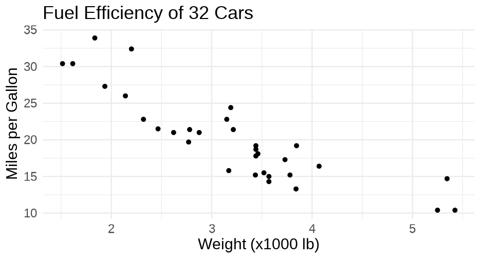

Support for lots of things!

Ligatures and font-awesome icons

library(ragg)
ggplot() + 
  geom_text(
    aes(x = 0, y = 2, label = "x <- y != z"), 
    family = "Fira Code"
  ) +
  labs(title = "twitter") +
  theme(plot.title = element_text(
      family = "Font Awesome 5 brands"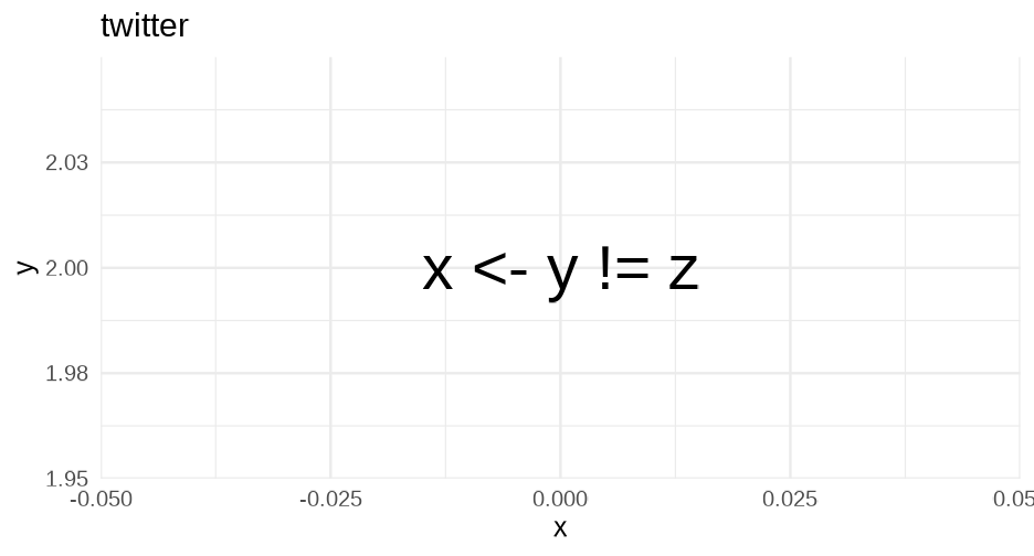
    )
  )

emojis

ggplot(mtcars, aes(disp, mpg)) +
  geom_text(label = "🎉",
            family = "Apple Color Emoji",
            size = 10)

Google fonts

https://fonts.google.com

• Open source, designed for the web

• Good place to explore fonts

• Can be incorporated via the {showtext} package!

{showtext} example

devtools::install_github("yixuan/showtext")
library(showtext)
font_add_google('Monsieur La Doulaise', "mld")
font_add_google('Special Elite', "se")
showtext_auto()
quartz()
ggplot(mtcars, aes(disp, mpg)) +
  geom_point() + 
  labs(title = "An amazing title", 
       subtitle = "with the world's most boring dataset") + 
  theme(plot.subtitle = element_text(size = 18, family = "se"),
        plot.title = element_text(size = 22, family = "mld"),
        axis.title = element_text(size = 18, family = "mld"),
        axis.text.x = element_text(size = 12, family = "se"),
        axis.text.y = element_text(size = 12, family = "se"))

Megaflicks

Quick aside

Change the font of your R Markdown!

Create a CSS code chunk - write tiny bit of CSS - voila!

@import url('https://fonts.googleapis.com/css?family=Akronim&display=swap');
body {
  font-family: 'Akronim', cursive;
}

Render!

Aside

I actually did this for these slides to make the tables a bit smaller!

Resource for learning more

• I'm not an expert on fonts. I have mostly just picked what looks nice to me.

Best I've heard of is practical typography

Identify fonts

Use others work to help you - I found the font for these slides from a different theme that I liked.

Use google chrome's developer tools to help!